Concept and theory of spatial interpolation #
Spatial interpolation is often used to convert discrete point measurement data into continuous data surfaces for comparison with other spatial phenomena distribution patterns, which includes both spatial interpolation and extrapolation algorithms. The spatial interpolation algorithm is a method for calculating data of other unknown points in the same region by using data of known points; the spatial extrapolation algorithm is a method for deriving data of other regions by using data of known regions. Spatial interpolation must be done in the following cases:
The resolution of existing discrete surfaces, the size or direction of pixels do not match the requirements, and need to be interpolated again. For example, a scanning image (aerial image, remote sensing image) is converted from one resolution or direction to another resolution or direction.
The existing data model of continuous surface does not conform to the required data model and needs to be interpolated again. For example, a continuous surface is changed from one spatial segmentation mode to another, from TIN to grid, grid to TIN or vector polygon to grid.
The existing data can not cover the required area completely, so interpolation is needed. For example, the discrete sampling point data are interpolated into a continuous data surface.
The theoretical hypothesis of spatial interpolation is that the nearer the point is, the more likely it is to have similar eigenvalues; and the farther the point is, the less likely it is to have similar eigenvalues. However, there is another special interpolation method - classification, which does not consider the spatial relationship between different types of measurements, only considers the average or median in the sense of classification, and assigns attribute values to similar objects. It is mainly used for the processing of equivalent regional maps or thematic maps of geology, soil, vegetation or land use. It is uniform and homogeneous within the “landscape unit” or patches, and is usually assigned a uniform attribute value, changes occur at the boundary.
Data source of spatial interpolation #
Data sources for continuous surface spatial interpolation include:
Orthophoto or satellite images obtained by photogrammetry;
Scanning images of satellites or space shuttles;
Sampling data are measured in the field. Sampling points are randomly distributed or regularly linearly distributed (along profiles or contours).
Digitized polygon maps and contour maps.
Spatially interpolated data is usually measured data of sampling points with limited spatial variation, these known measurement data are called “hard data”. If the sampling point data is relatively small, spatial interpolation can be assisted according to the known information mechanism of a natural process or phenomenon that causes some spatial change, this known information mechanism is called “soft information”. However, in general, due to the unclear mechanism of this natural process, it is often necessary to make some assumptions about the spatial variation of the attributes of the problem, such as assuming that the data changes between sampling points are smooth, and assuming that the relationship between distribution probability and statistical stability is obeyed.
The spatial position of the sampling points has a great influence on the results of spatial interpolation, ideally, the points are evenly distributed in the study area. However, when there are a large number of regular spatial distribution patterns in the regional landscape, such as regularly spaced numbers or ditches, it is clear that a completely regular sampling network will yield a one-sided result, for this reason, statisticians hope to pass some random sampling to calculate the unbiased mean and variance. But completely random sampling also has its drawbacks, firstly, the distribution of random sampling points is irrelevant, while the distribution of regular sampling points only needs a starting point, direction and fixed size interval, especially in complex mountains and woodlands. Secondly, completely random sampling will result in uneven distribution of sampling points, data density of some points, and lack of data of other points. Figure 8-15 lists several options for spatial sample point distribution. Fig. 125 Various sampling methods # 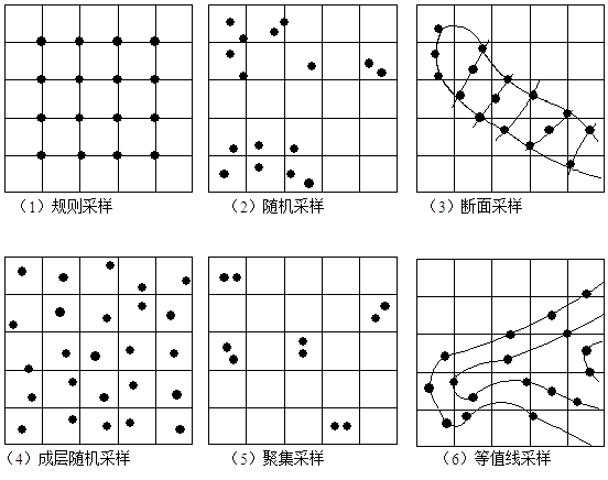
A good combination of regular sampling and random sampling is layered random sampling, that is, individual points are randomly distributed in the regular grid. Aggregated sampling can be used to analyze spatial variations at different scales. Regular cross-section sampling is often used to measure River and hillside profiles. Isoline sampling is the most commonly used method for digital contour interpolation of digital elevation model.
Term: A property value of a data point, which is one of all measurement points. It is the value of a point
x_0
after interpolation. If an interpolation method calculates data in which the calculated data of the sampling point is equal to the known sampling data, the interpolation method is called an exact interpolation method; all other interpolation methods are approximate interpolation methods, the difference between the calculated and measured values (absolute and squared), which is a commonly used indicator for evaluating the quality of inexact interpolation methods.
Spatial interpolation method #
Spatial interpolation methods can be divided into two categories: global interpolation and local interpolation. The global interpolation method uses the data of all the sampling points in the study area to fit the whole area features; the local interpolation method uses only the adjacent data points to estimate the value of the unknown points.
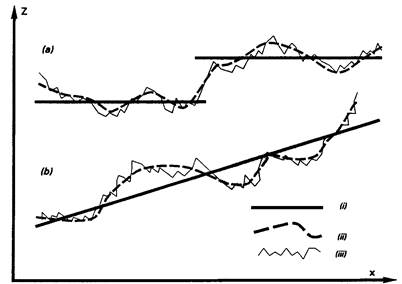
The global interpolation method is usually not directly used in spatial interpolation, but used to detect the largest deviation from the general trend. After removing the macroscopic features, the residual error can be used for local interpolation. Because the global interpolation method regards short-scale and local changes as random and unstructured noise, this part of information is lost. Local interpolation method can just make up for the defect of global interpolation method, and can be used for local outliers, and is not affected by interpolation of other points on the interpolation surface. 1) Boundary interpolation method The boundary interpolation method assumes that any significant changes occur at the boundary, and the changes within the boundary are uniform and homogeneous, that is, the same in all directions. This conceptual model is often used for soil and landscape mapping, and can be used to define other soil and landscape features by defining “homogeneous” soil units and landscape maps. The simplest statistical model for boundary interpolation is the standard variance analysis (ANOVAR) model: In the formula, The model assumes that the attribute values of each class k are normally distributed; the mean of each class k ( The index to evaluate the classification effect is that the smaller the ratio is, the better the classification effect is, for the variance between classes and for the total variance. In essence, the theoretical assumption of boundary interpolation method is: Attribute value Z varies randomly in “patches” or landscape units, but not regularly: All “patches” of the same category have the same class variance (noise); All attribute values are normal distribution; All spatial variations occur at the boundary and are sudden rather than gradual. When using boundary interpolation, careful consideration should be given to whether the data source conforms to these theoretical assumptions. 2) Trend surface analysis The continuous spatial variation of a geographical attribute can be described by a smooth mathematical surface. The approach involves first fitting a smooth mathematical surface equation using known sample point data, then applying this equation to estimate values at unmeasured points. This method, which relies solely on the relationship between attribute data of sample points and their geographic coordinates through multiple regression analysis to derive a smooth mathematical surface equation, is referred to as trend surface analysis. Its theoretical assumptions are that the geographic coordinates (x, y) are independent variables, the attribute value z is also an independent variable following a normal distribution, and similarly, the regression error is an independent variable unrelated to location. Polynomial regression analysis is the simplest method to describe the characteristics of long-distance gradual change. The basic idea of polynomial regression is to use polynomials to represent lines and surfaces, and to fit data points according to the principle of least square method. The choice of line or surface polynomials depends on whether the data is one-dimensional or two-dimensional. A simple example can be used to illustrate this: in geographical or environmental surveys, the characteristic value z is sampled at locations x_1 , x_2 , …, x_n along a transect. If the value of z increases linearly with x , the long-term change of this characteristic value can be calculated using the following regression equation: Where b 0 , b 1 is the regression coefficient, and ε is the normal distribution residual (noise) independent of x. However, in many cases, the quadratic polynomial is needed to fit the change in a more complex way rather than in a linear function: For the two-dimensional case, the surface polynomials obtained by the multivariate regression analysis of XY coordinates are as follows: The first three forms are: Plane Oblique plane Two degree surface Where P is the number of times of the trend surface equation. It is the minimum number of terms of trend surface polynomials under normal conditions. Zero degree polynomial is a plane with one item number; first degree polynomial is an oblique plane with three items number; quadric surface has six items number and cubic trend surface has 10 items number. The calculation factor b :sub:`i` is a standard multivariate regression problem. The advantages of trend surface analysis are very easy to understand, at least in terms of calculations. In most cases, low-order polynomials can be used for fitting, but it is more difficult to assign complex polynomial to explicit physical meaning. The trend surface is a smoothing function, it is difficult to pass the original data point. Unless the data point is small and the trend surface number is high, the surface just passes through the original data point, so the trend surface analysis is an approximate interpolation method. In fact, the most effective application of trend surface is to reveal the largest deviation from the general trend in the region, so the main purpose of trend surface analysis is to use trend surface analysis to remove some macroscopic features from the data before using a local interpolation method, instead of directly using it for spatial interpolation. As with multiple regression analysis, F distribution can be used to test the fitting degree of trend surface, and its test statistics are as follows: Where U is the sum of the squares of the regression, Q is the sum of the squares of the residuals (the sum of the remaining squares), p is the number of polynomial terms (excluding the constant term 3) Transform function interpolation The overall spatial interpolation based on empirical equations of one or more spatial parameters is also a frequently used spatial interpolation method, which is called a transformation function, the following is a description of a research example. Heavy metal pollution in alluvial plains is related to several important factors, of which the distance from the source (river) and the elevation are the most important. Generally, the coarse sediment carrying heavy metals is deposited on the river beach, and the fine sediment carrying heavy metals is deposited in low-lying areas which are easy to be flooded during the flood season. Where the frequency of floods is low, the sediment particles carrying heavy metals are relatively small and are lightly polluted. Since the distance and elevation from the river are relatively easy to obtain spatial variables, the spatial interpolation between the contents of various heavy metals and their empirical equations can be used to improve the prediction of heavy metal pollution. The form of the regression equation in this case is as follows: In the formula, z(x) represents the content (ppm) of a certain heavy metal, This regression model is often called a conversion function and can be calculated by most GIS software. The transfer function can be applied to other independent variables such as temperature, elevation, rainfall, and distance from the sea and vegetation can be combined into a function of excess water content, the geographic location and its attributes can be combined into as many regressions as possible into the required regression model and then spatially interpolated. However, it should be noted that the physical meaning of the regression model must be clear, it should also be noted that all regression transfer functions belong to approximate spatial interpolation. Global interpolation methods usually use standard statistical methods such as difference analysis and regression equation, and the calculation is relatively simple. Many other methods can also be used for global spatial interpolation, such as Fourier series and wavelet transform, especially for remote sensing image analysis, but they require a large amount of data. Local interpolation only uses adjacent data points to estimate the value of unknown points, including several steps: Define a neighborhood or search range; Search for data points that fall within this neighborhood; Choosing mathematical functions to express the spatial variations of these finite points; Assign values to the data points located within the regular grid cells. Repeat this step until all points on the grid have been assigned values. The following aspects should be paid attention to when using local interpolation method: the interpolation function used; the size, shape and direction of neighborhood; the number of data points; whether the distribution of data points is regular or irregular. 1) Nearest Neighbor Method: Thiessen Polygon Method Thiessen polygon (also known as Dirichlet or Voronoi polygon) uses an extreme boundary interpolation method, using only the nearest single point for region interpolation. Thiessen polygon divides the region into sub-regions according to the location of data points. Each sub-region contains a data point. The distance between each sub-region and its data points is less than any distance to other data points, and the data points in each sub-region are assigned. Connections connecting all data points form Delaunay triangle, which has the same topological structure as irregular triangle network TIN. In GIS and geographic analysis, Thiessen polygon is often used for fast assignment. In fact, an implicit assumption of Thiessen polygon is that the nearest meteorological station is used for meteorological data at any location. In fact, unless there are enough meteorological stations, this assumption is inappropriate, because precipitation, air pressure, temperature and other phenomena are continuously changing. The results obtained by Thiessen polygon interpolation method only occur on the boundary, and are homogeneous and unchanged within the boundary. 2) Moving average interpolation method: distance reciprocal interpolation The distance reciprocal interpolation method combines the advantages of the adjacent point method of Thiessen polygon and the gradient method of trend surface analysis, which assumes that the attribute value of the unknown point In the formula, the weight coefficient is calculated by a function, requiring that when [condition is met], it generally takes the form of reciprocal or negative exponential functions. Among these, the most common form is the inverse distance weighting function, expressed as follows: In the formula, x j for unknown points, x i for known data points. The simplest form of the weighted moving average formula is called linear interpolation, fhe formula is as follows: The distance reciprocal interpolation method is the most common method for GIS software to generate raster layers based on point data. The calculated value of the distance reciprocal method is susceptible to the cluster of data points. The calculation result often shows a “duck egg” distribution pattern with isolated point data significantly higher than the surrounding data points, which can be improved by dynamically modifying the search criteria during the interpolation process. 3) Interpolation method of spline function Before the computer was used to fit curves and data points, the plotter used a flexible curve gauge to fit smooth curves piecewise. The piecewise curves drawn by this flexible curve plan are called splines. The data points matched with splines are called pile points, and the position of the control curve is controlled by the pile points when drawing the curve. The curve drawn by the curve gauge is mathematically described by a piecewise cubic polynomial function with continuous first-order and second-order continuous derivatives at its junction. Spline function is a mathematical equation equivalent to flexible curve gauge in mathematics with a piecewise function. Only a few points can be fitted once, and at the same time, the continuity of the connection of curve segments can be ensured. This means that the spline function can modify the registration of a few data points without recalculating the whole curve. Trend surface analysis can not do this (Fig. 16). Fig. 126 Local Characteristics of Spline Functions # (a:当二次样条曲线的一个点位置变化时,只需要重新计算四段曲线; b: When one point of a spline curve changes, only two segments of the curve need to be recalculated. The general piecewise polynomial p(x) is defined as: p(x)=p_i (x) I < x < x_i+1 (iTunes 1, 2, 3… , kmur1) ( j=0, 1, 2, …, r-1; i=1, 2, … , k-1 ) `x_1`, …, `x_k-1` * divide the interval `[x_0, x_k]` into *k subintervals. These division points are referred to as “breakpoints,” and the points on the curve corresponding to these x -values are termed “knots.” The function p_i(x) is a polynomial of degree at most m . The r term is used to represent the constraints of the spline function: r=0 , no constraint; r=1 , the function is continuous and has no constraints on its derivative; r = m - 1 , and the interval [x_x_k] can be represented by a polynomial; r=m, with the most constraints. When m=1, 2, 3, the corresponding splines are linear, quadratic, and cubic spline functions, with derivative orders of 0, 1, and 2, respectively. Quadratic spline functions must have continuous first derivatives at each node, while cubic spline functions must have continuous second derivatives at each node. A simple spline with r=m has only k+m degrees of freedom. The case where r=m=3 holds special significance, as it represents a cubic polynomial, which was historically the first function to be termed a “spline function.” The term “cubic spline” is used in three-dimensional cases, where it is applied to surface interpolation rather than curve interpolation. Since the range of discrete subintervals is wide, it may be a digitized curve, alculating simple splines in this range will cause certain mathematical problems, therefore, in practical applications, B splines are used—a special kind Spline function. B splines are commonly used to smooth digitized lines before display, such as various boundaries on soil or geological maps, as traditional cartography typically aims to produce smoother curves. However, using B splines to smooth polygon boundaries also presents certain issues, particularly in the calculation of polygon area and perimeter, where the results may differ from those before smoothing. To sum up, spline function is piecewise function, only a few data points are used at a time, so the interpolation speed is fast. Compared with trend surface analysis and moving average method, spline function retains local variation characteristics. Both linear and surface spline functions are visually satisfactory. Some shortcomings of spline function are that the error of spline interpolation can not be estimated directly, at the same time, the problem to be solved in practice is the definition of spline blocks and how to assemble these “blocks” into complex surfaces in three-dimensional space without introducing any abnormal phenomena in the original surface. 4) Space autocovariance best interpolation method: Kriging interpolation Several interpolation methods introduced in the previous section have not been well solved, such as the control parameters of trend surface analysis and the weights of reciprocal distance interpolation methods, which have a great impact on the results. These problems include: The number of average data points needs to be calculated; How to determine the size, orientation, and shape of the search neighborhood for data points; Is there a better method for estimating weight coefficients than calculating simple distance functions? Error problems related to interpolation. To solve these problems, Georges Matheron, a French geomathematician, and D. G. Krige, a South African mining engineer, have studied an optimal interpolation method for mine exploration. This method is widely used in groundwater simulation, soil mapping and other fields, and has become an important part of GIS software geostatistical interpolation. This method fully absorbs the idea of geostatistics and considers that any attributes that change continuously in space are very irregular. It can not be simulated by simple smooth mathematical functions, but can be described appropriately by random surface. The spatial attributes of this continuity change are called “regional variables”, which can describe the index variables of image pressure, elevation and other continuity changes. This method of spatial interpolation using geostatistics is called Kriging interpolation. Geostatistical method provides an optimization strategy for spatial interpolation, that is, the dynamic determination of variables according to some optimization criterion function in the interpolation process. The interpolation methods studied by Matheron, Krige and others focus on the determination of weight coefficients, so that the interpolation function is in the best state, that is, to provide the best linear unbiased estimation of the variable value at a given point. The regional variable theory of Kriging interpolation assumes that the spatial variations of any variable can be expressed as the sum of the following three main components (Fig. 8-17): Structural components related to constant mean or trend; Random variables related to spatial change, i.e. regional variables; Spatially independent random noise or residual error terms. Fig. 127 Theory of regional variables divides complex spatial changes into three parts # Average characteristics of terrain; Spatially correlated irregular variations; Random and local variations In addition, x is a position in 1D, 2D or 3D space. The value of the variable z at x can be calculated as follows: In the formula, m (x) is a deterministic function describing the structural components of Z (x); a random variable related to spatial variation, i.e. a regional variable; and a residual error term with zero mean value and spatial independent Gauss noise term. The first step in the Kriging method is to determine the appropriate m(x) function. In the simplest case, m(x) is equal to the average of the sampling area, and the distance vector h is separated. The mathematical expectation between two points x , x+h is equal to zero: Where z(x) , z(x+h) is the value of the random variable z at x, x+h , and also assumes that the variance between the two points is only Related to distance h , then: In the formula, it is a kind of function, called semi-variance function. The two inherent assumptions of regional variable theory are the stability and variability of differences. Once the structural components are determined, the remaining differences belong to homogeneous changes, and the differences between different locations are only functions of distance. In this way, the formula for calculating regional variables can be written in the following form: The estimating formulas of semi-variance are as follows: In the formula, n is the number of sample point pairs with distance h ( n to point), and the sampling interval h is also called delay. The map corresponding to h is called the “half variance graph”. Figures 8-18 show a typical half-variance plot. Semivariance is the first step in quantitatively describing regionalized variation, providing valuable information for spatial interpolation and optimizing sampling schemes. To obtain a semivariogram, a theoretical model fitting the semivariance must first be established. In the theoretical model of semivariance: The part of the curve with the larger value of delay h is horizontal, the horizontal part of the curve becomes “Sill”. Note that there is no spatial correlation of data points in this range of delays because all variances do not change with distance. The delay range of curve from low value to beam is called Range. The range is the most important part of the semivariogram because it describes how space-related differences vary with distance. The closer the distance is within the range of the range, the more similar features are. The range provides a way to determine the size of the window for the moving weighted averaging method. Obviously, the distance between the data point and the unknown point is greater than the range of the range, indicating that the data point is too far away from the unknown point and has no effect on the interpolation. The fitting model in the graph does not pass through the origin, but is intersected with the coordinate axis in the positive direction. Fig. 128 Semivariogram # According to the semivariance formula, when h = 0, it must be zero. The positive value appearing in the model is the estimated value of residual error, which is space-independent noise. Called “Nugget” variance, it is a combination of observation errors and spatial variations with small distance intervals. When there are obvious ranges and beams, and the kernel variance is also important, but the numerical value is not too large, the spherical model can be used to fit the semivariance (Figure 8-19-1). The formula is: 0 < h < a h >= a h=0 In the formula, A is a variable, h is a delay, The exponential model (Figure 8-19-2) can be used for fitting if there are obvious kernel variances and beams without gradual variation: When the nugget variance is significantly smaller than the random variation associated with spatial variation, it is preferable to use a more curved curve, such as the Gaussian curve (Figure 8-19-4). If the spatial variation varies with the range, but there are no beams, the linear model (Figure 8-19-3) can be used to fit: In formula B is the slope of the line. Linear models are also used when the range of variation is much larger than the desired interpolation range. Previous discussions assume that the surface features are identical in all directions, but in many cases, spatial variations have obvious directivity, which requires the use of models with different parameters to fit semivariance maps. Fig. 129 Various types of variograms # The fitted semivariogram serves an important purpose in determining the weighting factors required for local interpolation. The determination process is similar to the weighted moving average interpolation method, but instead of being calculated using a fixed function, it is computed based on the statistical analysis principles of the sampled data’s semivariogram. That is: The selection of weights should be unbiased and the variance of the estimation is less than that of other linear combinations of observations. The minimum variance is: The minimum variance that can only be obtained when the following equation holds: The semi-variance between x_j points; specifically, the semi-variance between the sample point x_j and the unknown point x_0 . Both of these quantities can be obtained from the fitted model’s semi-variogram. Calculate the Lagrangian multiplier required for minimizing the variance. This method is called conventional Kriging interpolation. It is an exact interpolation model, and the interpolation or the best local mean is consistent with the data points. In cartography, regular grids with thinner sampling intervals are often used for interpolation, which can be converted into contour maps by the methods mentioned above. Similarly, the estimated error, also known as Kriging variance, can be used to map the reliability of interpolation results throughout the study area. An example of Kriging interpolation: (Figure 8-20) Fig. 130 An example of Kriging interpolation # Calculate the weight of the kriging method of the unknown point I0 in the graph (x=5, y = 5), and use the spherical model to fit the semivariance, parameter I x y z I1 2 2 3 I2 3 7 4 I3 9 9 2 I4 6 5 4 I5 5 3 6 The solution process is represented by a matrix as follows: Where A is the semivariance matrix between the data points, b is the semivariogram vector between each data point and the unknown point, λ is the weight coefficient vector to be calculated, Φ is the solution equation Lagrange operator. Firstly, the distance matrix between the five data points is calculated: And the distance vectors between them and unknown points: Substitute the above values into the spherical model to obtain the corresponding semi-varances (matrix A, b): Note that the additional sixth row and sixth column are included to ensure the sum of the weights equals 1. By calculating the inverse matrix of A, the following results are obtained: A:sup:`-1`= I 1 2 3 4 5 6 1 -0.172 0.050 0.022 -0.026 0.126 0.273 2 0.050 -0.167 0.032 0.077 0.007 0.207 3 0.022 0.032 -0.111 0.066 -0.010 0.357 4 -0.026 0.077 0.066 -0.307 0.190 0.030 5 0.126 0.007 -0.010 0.190 -0.313 0.134 6 0.273 0.207 0.357 0.003 0.134 -6.873 Thus, the weight λ is: I weight coefficient distance 1 0.0175 4.423 2 0.2281 2.828 3 -0.0891 ∑ = 1 5.657 4 0.6437 1.000 5 0.1998 2.000 6 0.1182 φ The interpolated value at the unknown point is: z(I0) =0.0175*3 + 0.2281*4 - 0.0891*2 + 0.6437*4 + 0.1998*6 = 4.566 The estimated variance is: σ_e_2 = [0.0175 7.151+ 0.2281* 5.597 - 0.0891*8.815* + 0.6437*3.621 + .1998*4.720 ] +φ = 3.890 + 0.1182 = 4.008 The purpose of the Kriging interpolation method is to provide a method for determining the optimal weight coefficient and to describe the error information. Since the interpolation value of the Kriging point model (conventional kriging model) is related to the capacity of the original sample, when the sample is small, the interpolation result graph with simple point conventional Kriging interpolation will have obvious unevenness. This shortcoming can be overcome by modifying the Kriging equation to estimate the average within the sub-block B , this method is called block Kriging interpolation, which is suitable for estimating the average of a given area test cell or interpolating a regular grid of a given grid size. The mean value of Z in subblock B is: In the formula, S_B represents the area of subregion B. The same estimation formula continues to be used for z(x): The minimum variance is still: However, the conditions for its establishment are as follows: The variance of block Kriging interpolation is usually smaller than that of point Kriging interpolation, so the smooth interpolation surface generated will not produce concave and convex phenomena of point model. In recent years, Geographic Information Systems (GIS) have undergone rapid development in both theoretical and practical dimensions. GIS has been widely applied for modeling and decision-making support across various fields such as urban management, regional planning, and environmental remediation, establishing geographic information as a vital component of the information era. The introduction of the “Digital Earth” concept has further accelerated the advancement of GIS, which serves as its technical foundation. Concurrently, scholars have been dedicated to theoretical research in areas like spatial cognition, spatial data uncertainty, and the formalization of spatial relationships. This reflects the dual nature of GIS as both an applied technology and an academic discipline, with the two aspects forming a mutually reinforcing cycle of progress.Global interpolation method #
z
is the attribute value at position
x_0
,
μ
is the population mean,
α_k
is the difference between the mean of class
k
and
μ
, and
ε
is the average within-class error (noise).
μ+α_k
) is estimated from an independent sample set and is assumed to be spatially independent; the average error
ε
between classes assumes that all classes are identical.
F
test can be used to test the significance of classification results.
b_0
), and n is the number of data points used. When
F>F_a
, the trend surface is significant, otherwise it is not significant.
b_0
…
b_n
are regression coefficients, and
p_1
…
p_n
are independent spatial variables. In this example,
p_1
is the distance-to-river factor, and
p_2
is the elevation factor.Local interpolation method #
x_0
is the distance weighted average of all data points in the local neighborhood. The distance reciprocal interpolation method is one of the weighted moving average methods, the weighted moving average method is calculated as follows: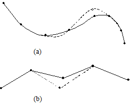
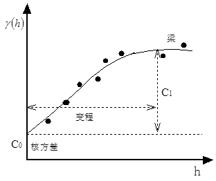
c_0+c_1
is the beam. Generally, the fitting effect of spherical model is ideal.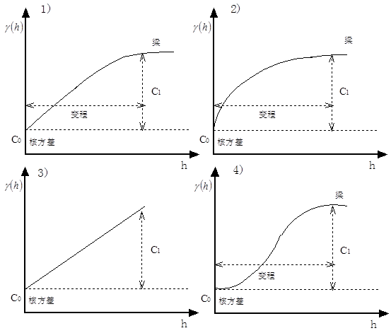
x_i
.
       c_0=
       2.5
,
       c_1
       =7.5
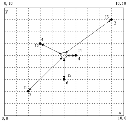
; range a = 10.0. The data of these 5 sampling points are:*I 1 2 3 4 5*
*I1 0.0 5.099 9.899 5.000 3.162*
*I2 5.099 0.0 6.325 3.606 4.472*
*I3 9.899 6.325 0.0 5.0 7.211*
*I4 5.0 3.606 5.0 0.0 2.236*
*I5 3.162 4.472 7.211 2.236 0.0 *
*I I0*
*I1 4.243*
*I2 2.808 *
*I3 5.657 *
*I4 1.0*
*I5 2.0*
*A= I 1 2 3 4 5 6*
*1 2.500 7.739 9.999 7.656 5.939 1.000*
*2 7.739 2.500 8.677 6.381 7.196 1.000*
*3 9.999 8.677 2.500 7.656 9.206 1.000*
*4 7.656 6.381 7.656 2.500 4.936 1.000*
*5 5.939 7.196 9.206 4.936 2.500 1.000*
*6 1.000 1.000 1.000 1.000 1.000 0.000*
*b = I 0 *
*1 7.151*
*2 5.597*
*3 8.815*
*4 3.621*
*5 4.720*
*6 1.000*