For simulating phenomena with continuous spatial distribution, the field-based view is appropriate, such as the concentration of pollutants in the air, the surface temperature, the soil moisture level, the velocity and direction of air and water flow. According to the different applications, the field can be expressed as two-dimensional or three-dimensional. A two-dimensional field is a value representing this phenomenon at any known location in a two-dimensional space. A three-dimensional field is a value for any location in a three-dimensional space. Some phenomena are essentially three-dimensional in space, such as air pollutants, but in many cases it can be represented by a two-dimensional field.
The field model can be expressed as the following mathematical formulas:
In the upper expression, z is the measurable function, s is the position in the space, so the expression represents the mapping from the space domain (even including the time coordinates) to a value domain. Some common models examples are given in geographic research [A. Vckovski] (Table 3-1).
Field model | Definition domain dimension | Range dimension | Independent variable | Dependent variable |
|---|---|---|---|---|
T(z) | 1 | 1 | Space coordinates (Elevation) | Temperature at altitude-Z |
E(t) | 1 | 3 | Time coordinate | Electrostatic force at a certain moment |
H (x, y) | 2 | 1 | Spatial coordinates | Surface elevation |
P (x, y, z) | 3 | 1 | Spatial coordinates | Soil porosity |
v(λ,φ,z) | 3 | 3 | Space coordinates (λ, φlatitude and longitude, z height) | Wind speed (three-dimensional vector) |
σ(x,y,z) | 3 | 9 | Spatial coordinates | Pressure tensor |
Θ(λ,φ,p,t) | 4 | 1 | p pressure surface, t time | Latent temperature |
Θ:sub:`t`(λ,φ,p) | 3 | ∞ | p pressure surface | Potential temperature over time |
I (x, y, z, t, λ) | 5 | 1 | x, y, z, t space-time coordinates, wavelength of λ | Radiation intensity of electromagnetic wave with wavelength λ at x, y, z, t |
Field characteristics #
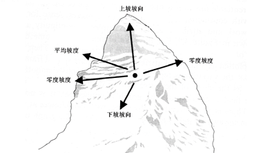
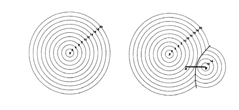
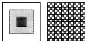
Field is often considered to consist of a series of contours, a contour is an ordered set of all points on the ground with the same attribute values. In practical applications, “space” often refers to Euclidean space that can be measured in length and angle. Spatial structures can be regular or irregular, but the resolution and position errors of spatial structures are very important. They should be compatible with the data types and analysis supported by spatial structure design. The values of the property fields can be divided into the following types: name, ordinal number, interval, and ratio. Another feature of attribute fields is that supported null values, and null values are assigned if the values are unknown or uncertain. If the functions in the spatial domain are continuous, the spatial domain is also continuous. With the slight change of the spatial position, the attribute values will also change slightly, and there will be no sudden change like the cliff in the digital elevation model. Only defined “small change” in the spatial structure and attribute domain, the “continuity” also be properly defined; When the spatial structure is two-dimensional (or more dimensions), the gradient( or rate of change) depends not only on the particular location, but also on the direction distribution of the region where the location is located (Fig. 3-2). There is a logical relationship between the two concepts of continuity and differentiability. Each differentiable function must be continuous, but the continuous function is not necessarily differentiable. Fig. 28 The slope at a given point is determined by the differentiability of the terrain in all directions at that location # If the spatial domain function is differentiable, the spatial domain is differentiable. The boundary change of administrative divisions is an example of discrete. If the boundary measured at present is located in A, and the boundary at this time last year is located in B. This does not mean that the boundary will be at the center between B and A before six months, and the boundary has discontinuous jump. It is an important characteristic of space field whether the properties of space field change with the direction. If all properties in a field are independent of direction, they are called isotropic fields. For example, if the travel time from one point to another is only proportional to the Euclidean geometric distance between the two points, then it starts from a fixed point that can be reached by a certain time of travel, it must be an isochronal circle, as shown in Figure 3-3-(a). If there is a high-speed channel at a certain point, the travel time generated by using and not using the high-speed channel is different, as shown in Figure 3-3-(b). The isochron has been marked in the figure. The hyperbola in the figure is the boundary between using and not using high-speed channels. In this case, the travel time is related to the orientation of the target point and the starting point, which is called the Anisotropic Field. Fig. 29 Travel time surface in isotropic and anisotropic fields # Spatial autocorrelation is a measure of the degree of numerical aggregation in a spatial field. The connection between things near is stronger than that between things far away. If similar values in a spatial field tend to aggregate, the spatial field shows a strong positive spatial autocorrelation. If similar attribute values tend to repel each other in space, they show negative spatial autocorrelation (Figure 3-4). Therefore, spatial autocorrelation describes the relationship between attribute values at a location and those at adjacent locations. Fig. 30 Strong Spatial Positive and Negative Autocorrelation Model # Spatial structural features and attribute domains #
Continuous, differentiable and discrete #
Direction-independent and direction-related (isotropy and anisotropy) #
Spatial autocorrelation #
Raster Data Model #
The raster data model is based on continuous tessellation, which discretizes continuous space by covering the entire area with a two-dimensional grid or partition. Tessellations can be regular or irregular, with the latter often represented as topological polygons, such as socioeconomic zones or urban blocks. Key characteristic parameters of a tessellation include cell size, shape, orientation, and spacing. For the same geographic phenomenon, multiple tessellations may exist at different scales and levels of aggregation or subdivision. Among regular tessellations with polygon side counts ranging from 3 to N, squares, triangles, and hexagons are the most commonly used in spatial data processing. The triangle serves as the most fundamental indivisible unit, capable of assuming different forms based on angle and side length variations. Notably, squares, triangles, and hexagons possess the geometric property of being able to completely tile a plane without gaps or overlaps (Figure 3-5). Fig. 31 Partition of triangle, grid and hexagon # 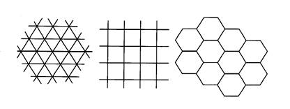
The spatial model based on raster considers space as a test sellation of Pixel. Each pixel is related to a record of the phenomena contained in the classification or identification. Pixel and raster are both content from image processing, in which a single image can be generated by scanning each raster. Raster data in GIS are often from artificial and satellite remote sensing scanners, as well as devices used for digital files. Information systems using raster models usually employ the hierarchical approach described above. In each layer, raster pixels record the existence of special phenomena. The values of each pixel indicate the classification of phenomena in a given class (Fig. 3-6). Fig. 32 Raster Data Model # 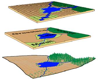
Because the pixels have fixed size and location, the grid tends to be a natural and artificial phenomenon in a “grid block”. Therefore, the boundaries between classifications are forced to use the boundaries along the grid pixels. Each pixel in a raster layer is usually divided into a single type. This may lead to a misunderstanding of the distribution of phenomena, depending on the size of the relevant pixels. If the pixels are very small for features, the grid can be a particularly effective way to represent the random distribution of the boundary of natural phenomena, which tend to gradually combine with each other rather than simply partition. If each pixel is limited to a class, the raster model can not adequately represent the transformation attributes of some natural phenomena. Unless sampling is reduced to a micro level, many data classes are in fact mixed classes. Fuzzy features can be effectively expressed in a grid by mixing pixels, where component classification is expressed by the percentage of all components measured or predicted. Nevertheless, it should be emphasized that the pixels of a grid are assigned only a single value.
For GIS data processing, an important feature of raster model is that the location of pixels in each predefined raster , so it is easy to overlap operations to compare the features stored in different layers. Because the location of pixels is predefined and identical in different layers of a specific application, each attribute can be logically or algorithmically combined with the attributes of the pixels in other layers to produce an attribute value in the corresponding overlap. It differs from the layer-based vector model in that the surface units in the layer are independent of each other, and the direct comparison of layers must be further processed to identify overlapping attributes.
Voxels: The raster representation based on GIS can be extended to three-dimensional to generate a Voxel model, in which the pixels are rectangular, typically consisting of cubes and three-dimensional elements. Some types of geographic data are not always represented by boundaries, because data values may be associated with an attribute that varies with location and does not clearly understand boundaries. A suitable model for data of this kind of model is the voxel model. This model is widely used in media imaging, which originates from computer-aided tomography (CT) and nuclear magnetic resonance scanner. They are good at representing progressive and special position changes and are suitable for profiles that produce such changes.