Three Ground Object Elements in Euclidean Space and Euclidean Space #

Many geographic phenomena are modeled by embedding them within a coordinate space where distances and directions between points can be measured using standard mathematical formulas. This coordinated spatial framework, known as Euclidean space, transforms spatial properties into tuples of real numbers.

The two-dimensional model is referred to as the Euclidean plane. In Euclidean space, the most commonly used reference system is the Cartesian coordinate system, defined by a fixed, distinctive point known as the origin and a pair of mutually perpendicular lines passing through this origin that serve as the coordinate axes. Additionally, other coordinate systems, such as the polar coordinate system, are also frequently employed in certain contexts.

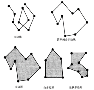
By embedding geographic elements into Euclidean space, three kinds of objects of ground objects are formed, namely point objects, line objects and polygonal objects.

Polygon objects #

Planar entities, also known as polygons, are descriptions of lakes, islands, land masses and other phenomena. Usually, it is represented by a closed curve and an interior point in the database. Planar entities have the following spatial characteristics:

• Area range;

• Perimeter;

• Independent or adjacent to other objects, such as China and its surrounding countries;

• Internal islands or serrated shapes, such as areas enclosed by closed coastlines of islands, etc;

• Overlapping and non-overlapping, such as the sales of newspapers, the division of schools, the service scope of the vegetable market may overlap. Generally speaking, each urban area of a city is adjacent but does not overlap.

In computational geometry, many different types of polygons are defined as shown in Figure 3-7.

Basic concepts of factor model #

Element-based spatial models emphasize individual phenomena, which are studied independently or in a way that correlate with other phenomena. Any phenomenon, regardless of size, can be identified as an object, assuming that it can be conceptually separated from its neighborhood phenomena. Elements can be composed of different objects, and they can have special relations with other separated objects. In an application related to the owner record of land and property, a factor-based perspective is adopted, because each land block and each building must be different and must be uniquely identified and can be measured individually. A factor-based view is appropriate for organized boundary phenomena, although not limited. Therefore, it is also suitable for man-made phenomena, such as buildings, roads, facilities and management areas. Some natural phenomena, such as lakes, rivers, islands and forests, are often represented in factor-based models because they can be seen as discrete phenomena for certain purposes, but it should be remembered that the boundaries of such phenomena are seldom fixed over time, so their actual location definitions are seldom accurate at any time.

The element-based spatial information model decomposes the information space into objects or entities. An entity must meet three conditions:

• It can be identified;

• Important (related to the problem);

• It can be described (characterized).

The characteristics that related entities can be described by static attributes (such as city names), dynamic behavior characteristics and structural characteristics. Unlike the field-based model, the factor-based model regards the information space as a collection of many objects (cities, towns, villages, districts), which have their own attributes (such as population density, centroid and boundary). The entities in the element-based model can define attributes in many dimensions, including spatial dimension, temporal dimension, graphic dimension and text/digital dimension.

Spatial objects are designated as “spatial” because they are embedded within a space. The definition of a spatial object depends critically on the structure of this embedding space. Common types of embedding spaces include:

1. Euclidean space, which allows for the measurement of distance and direction between objects, enables the representation of these objects as collections of coordinate tuples;

2. A metric space is defined as a set in which a distance measure can be applied between objects, but not necessarily direction;

3. A topological space is defined as a set in which topological relationships between objects can be described, without necessarily having defined concepts of distance or direction;

4. A set-oriented space is defined as a space that utilizes only fundamental set-based relations, such as containment, union, and intersection.

1) Types of Spatial Objects on Euclidean Plane

It shows a possible hierarchy of object inheritance on a continuous two-dimensional Euclidean plane(Figure 3-8).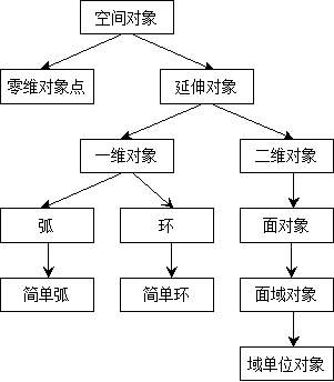

The object with the highest abstraction level is the “space object” class, which derives from zero-dimensional point and extended objects which can derive from one-dimensional and two-dimensional object classes (the above figure). Two subclasses of one-dimensional objects: arc and ring (Loop), if they do not intersect, they are called Simple Arc and Simple Loop. In the two-dimensional space object class, the connected object is called the area object, and the simple area object without “hole” is called the area unit object.

2) Spatial Objects on Discrete Euclidean Planes

The Euclidean plane, by its continuous nature, is not directly computable and must be discretized to become tractable for computational purposes. All continuous types discussed have their discrete counterparts, as shown in Figure 3-8. Figure 3-9 illustrates a partial inheritance hierarchy of discrete one-dimensional objects.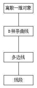

Object behavior is defined by some operations. These operations are used for one or more objects (operation objects) and produce a new object (result). Spatial operations acting on spatial objects can be divided into two categories: static and dynamic. Static operations do not lead to essential changes in operational objects, while dynamic operations change (or even generate or delete) one or more operational objects.

Although the system’s object-oriented method and element-based spatial data model are similar in concept, there are still obvious differences between them. The implementation of factor-based models does not necessarily require the use of object-oriented methods; on the other hand, object-oriented methods can be used as a framework for describing both the spatial model of the field and the spatial model based on the elements. For element-based models, object-oriented description is obviously appropriate. For field-based models, object-oriented method can also be used to build.

Fields and objects can coexist at many levels. For spatial data modeling, field-based methods and element-based methods are not mutually exclusive. Some applications can naturally apply field modeling to establish field models, such as the climate change in a region mentioned in the previous example. However, even in this case, field models are not suitable for all situations. For example, if the points collecting rainfall data are scattered and irregularly distributed in space, and these points have their own characteristics, then an object may be more suitable for describing the changes of regional climate attributes, containing two attributes, location and average rainfall. In a word, the field-based model and the factor-based model have their own advantages. They should be properly integrated to model. In the high-level modeling of GIS application model, data structure design and GIS application, the integration of these two models will be encountered. Figure 3-10 depicts the comparison between the element model and the field model.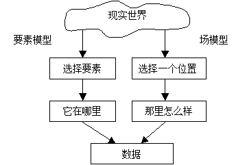

Vector Data Model #

Vector method (Fig. 3-11) emphasizes the existence of discrete phenomena. The boundary is determined by boundary lines (points, lines and surfaces), so it can be seen as element-based. However, in some vector-based GIS, the convenience of surface representation brings the possibility of simulating two-dimensional field. The most common example is surface elevation. Grid technology is often described as location-based because it focuses on the content of the location of spatial grid pixels. The raster data model seems to be similar to the field view, but the stored spatial information model is not a description of a continuous variable. A set of grid-pixel values, which can certainly be regarded as sampling a field model can also be sampled as an object-based model.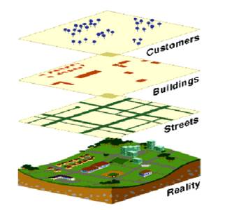

Vector data model regards phenomena as a set of primitive entities and constitutes spatial entities. In the two-dimensional model, the prototype entity is point or line or surface. In the three-dimensional model, the prototype also includes surface and body. The scale of observation or the degree of generalization determine the type of prototype. In a small scale representation, phenomena such as towns can be represented by individual points, while roads and rivers are represented by lines. When the scale of performance increases, the scale of phenomena must be taken into account. On a medium scale, a town can be represented by a specific prototype, such as a line, to record its boundaries. On a larger scale, towns will be represented as a complex collection of specific prototypes, including building boundaries, roads, parks and other natural and management phenomena.

The expression of vector model originates from the prototype space entity itself, which is usually defined by coordinates. The position of a point can be described by a single set of coordinates in two or three dimensions. A line is usually represented by an orderly set of two or more coordinate pairs. The path of a line between specific coordinates can be a linear function or a higher mathematical function, and the line can be determined by the set of intermediate points. A surface is usually defined by a boundary, which consists of one or more lines forming a closed ring. If there is a hole in the region, then multiple rings can be used to describe it.

Depending on the type of application, there are specific requirements for using vector data to describe three-dimensional models. For terrain modeling applications, the requirement is either for a simple, single-valued surface, meaning that for any given location, there is a single, definite elevation value, which can only represent surface elevation; or they are combined with the topographic features of the terrain surface. In landscape architecture, it is necessary to integrate the terrain surface with three-dimensional representations of features, such as buildings and vegetation located on it. For cartographic purposes, the traditional method of representing terrain surfaces uses contour lines, but for analytical purposes, contour lines are not a convenient representation. If the surface is sampled as isolines (perhaps digitized from a map), they are usually converted into the most common GIS-based terrain representations, such as regular grids and triangulated irregular networks (TIN). A regular grid of point values, or a matrix, can be derived directly from an original regular sampling scheme, but more commonly, it is generated by interpolating irregularly distributed values, which may include digitized contour lines and discrete point elevation values. A key characteristic of TINs is that they preserve the original irregularly sampled data values; it is a triangulation used to represent a surface with triangular planes connected to these original values. The surface of a TIN facet is typically considered planar by default, but curved interpolation functions can also be applied between vertices.

If TIN is used to represent a single value surface (whether terrain data or other), it provides a digital representation of a two-dimensional field when combined with an interpolation function. Similarly, if a grid of sampling points is accompanied by an interpolation function between sampling points, it can also be used to implement a field model.

If volume objects are stored in vector-based GIS, they are usually defined by one or more closed surfaces, while surfaces can be defined by polygons surrounded by three-dimensional lines. Lines and their constituent points, or sets of vertices, define such surfaces as a polygonal mesh structure. Each surface of the net is considered to be flat or curved; in both cases, a mathematical function is needed to indicate the position of the surface between specific coordinates. If a smooth surface is needed, the digital surface function can be constructed by the vertices of the polygonal network, then the computer graphics display of such a surface can be realized by decomposing the digital surface into very small planes. Examples of mathematical surface functions are B-spline functions. These types of functions control the relationship between the known control points and the fitted surface, including the measurement of the surface and the approximation between the control points and the fitted surface.