1.Python processing raster image

1.1 Read tif

import rasterio
from rasterio.plot import show
from matplotlib import colors, cm
rs = rasterio.open(r'C:\Users\lenovo\Desktop\pzh_map_dispose\sf1.tif','r')
result1=rs.read()

1.2 Replace Nodata data

#If the conditions are met, replace it; otherwise, keep it as it is
result=np.where(result1==result1.min(),np.nan,result1)
result
# np.unique(rss[0])

out:

array([[[nan, nan, nan, ..., nan, nan, nan],

[nan, nan, nan, ..., nan, nan, nan],
[nan, nan, nan, ..., nan, nan, nan],
...,
[nan, nan, nan, ..., nan, nan, nan],
[nan, nan, nan, ..., nan, nan, nan],
[nan, nan, nan, ..., nan, nan, nan]]])

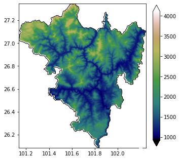
1.3 Display TIF

import geopandas as gpd
shp = gpd.read_file(r"C:\Users\lenovo\Desktop\pzh_map_dispose\pzh_city.shp")
fig, ax = plt.subplots(figsize=(5,9))
shp.plot(ax=ax,color='none')
show(result, transform=rs_mask.transform,ax=ax, cmap='gist_earth')
fig.colorbar(cm.ScalarMappable(norm=colors.Normalize(vmin=np.nanmin(result), vmax=np.nanmax(result)), cmap='gist_earth')
             , ax=ax,extend='both',fraction=0.05)

2.An example from scratch - full version

2.1 Create shp faces and write files

import os
import geopandas
from shapely import geometry
import matplotlib.pyplot as plt
x1,y1=30,30  
x2,y2=50,50
# Corresponds to Polygon in shapely.geometry, which is used to represent faces. Next, we create a polygon object composed of several Polygon objects
cq = geopandas.GeoSeries([geometry.Polygon([(x1,y1), (x2,y1), (x2,y2), (x1,y2)]),
                          geometry.Polygon([(x2,y1),(55,40), (x2,y2)])
                          ],
                         index=['1', '2'],  # Build an index field
                         crs='EPSG:4326',  # The coordinate system is WGS 1984
                         )
cq.to_file(r'simple_poly.shp',
           driver='ESRI Shapefile',
           encoding='utf-8')
cq

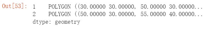
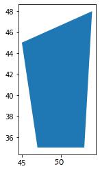
2.2 Read using geopandas

gdf=geopandas.read_file(r'simple_poly.shp')
gdf
gdf.plot(column='index')

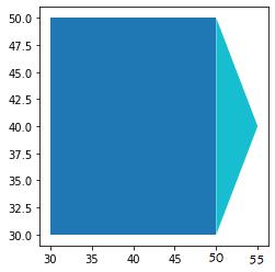
2.3 Convert to grid - convert to grid according to field

# Vector data to grid: no template required
def shpToRaster2(shp_path,raster_path,cellsize,field):
    '''
    Vector data to grid: No template required
    :param shp_path:Vector data to be converted
    :param raster_path:Grid save path after export
    :param cellsize:Cell size
    :param field:Vector data field as grid value
    :return:
    '''
    shp = ogr.Open(shp_path)
    m_layer = shp.GetLayer()
    extent = m_layer.GetExtent()    
    Xmin = extent[0]    
    Xmax = extent[1]    
    Ymin = extent[2]    
    Ymax = extent[3]  
    rows = int((Ymax - Ymin)/cellsize);    
    cols = int((Xmax - Xmin) / cellsize);    
    GeoTransform = [Xmin,cellsize,0,Ymax,0,-cellsize]    
    target_ds = gdal.GetDriverByName('GTiff').Create(raster_path, xsize=cols, ysize=rows, bands=1, eType=gdal.GDT_Float32) 
    target_ds.SetGeoTransform(GeoTransform)        target_ds.SetProjection(str(pro)) # Get projection must be converted to string  
    band = target_ds.GetRasterBand(1)
    pro = m_layer.GetSpatialRef()

    band.SetNoDataValue(-999)    
    band.FlushCache()
    # target_ds.SetProjection('GEOGCS["GCS_China_Geodetic_Coordinate_System_2000",DATUM["China_2000",SPHEROID["CGCS2000",6378137,298.257222101]],PRIMEM["Greenwich",0],UNIT["degree",0.0174532925199433,AUTHORITY["EPSG","9122"]],AXIS["Latitude",NORTH],AXIS["Longitude",EAST]]')    gdal.RasterizeLayer(target_ds, [1], m_layer, options=["ATTRIBUTE=%s"%field,'ALL_TOUCHED=TRUE'])  # Assign value to grid pixel with shp field
    del target_ds
    shp.Release()
    vector_fn=r'simple_poly.shp'
    raster_fn=r'two_region.tif'
    shpToRaster2(vector_fn,raster_fn,cellsize=0.5,field='index')

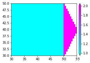
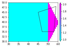
2.4 Display raster image

def showraster(inputtif): import rasterio from rasterio.plot import show from matplotlib import colors, cm rs =rasterio.open(inputtif)
rss=rs.read() #If the conditions are met, replace it; otherwise, keep it as it is result=np.where(rss==rss.min(),np.nan,rss) fig, ax = plt.subplots(figsize=(4,4)) show(result, transform=rs.transform,ax=ax, cmap='cool') from mpl_toolkits.axes_grid1 import make_axes_locatable divider = make_axes_locatable(ax) cax = divider.append_axes("right", size="3%", pad=0.1) # world.plot(column='pop_est', ax=ax, legend=True, cax=cax) fig.colorbar(cm.ScalarMappable(norm=colors.Normalize(vmin=np.nanmin(result), vmax=np.nanmax(result)), cmap='cool') , ax=ax,extend='both',fraction=0.010,cax=cax) return fig,ax showraster(r'two_region.tif')

2.5 Create a mask shape

import os
import geopandas
from shapely import geometry
import matplotlib.pyplot as plt
# Corresponds to Polygon in shapely.geometry, which is used to represent faces. Next, we create a polygon object composed of several Polygon objects
cq = geopandas.GeoSeries(geometry.Polygon([(47,35),(53,35),(54,48),(45,45)]),
                         index=['1'],  # Build an index field
                         crs='EPSG:4326',  # Coordinate system: WGS 1984
                         )
cq.to_file(r'simple_mask.shp',
           driver='ESRI Shapefile',
           encoding='utf-8')
gdf=geopandas.read_file(r'simple_mask.shp')
gdf.plot()

2.6 Simultaneous display

def showraster2(inputtif,inputshp):
    import rasterio
    from rasterio.plot import show
    from matplotlib import colors, cm
    rs =rasterio.open(inputtif)   
    rss=rs.read()
    #If the conditions are met, replace it; otherwise, keep it as it is
    result=np.where(rss==rss.min(),np.nan,rss)
    shp = gpd.read_file(inputshp)
    fig, ax = plt.subplots(figsize=(4,4))
    shp.plot(ax=ax,color='none')
    show(result, transform=rs.transform,ax=ax, cmap='cool')
    from mpl_toolkits.axes_grid1 import make_axes_locatable
    divider = make_axes_locatable(ax)
    cax = divider.append_axes("right", size="3%", pad=0.1)
    # world.plot(column='pop_est', ax=ax, legend=True, cax=cax)    
    fig.colorbar(cm.ScalarMappable(norm=colors.Normalize(vmin=np.nanmin(result), vmax=np.nanmax(result)), cmap='cool', ax=ax,extend='both',fraction=0.010,cax=cax))                ​​​​​​​

2.7 Mask extraction

# Use the mask above to extract the grid
def shp_mask(inputtif,inputshp,outtif):
    import fiona
    import rasterio
    import rasterio.mask
    rs = rasterio.open(inputtif,'r')
    with fiona.open(inputshp, "r") as shapefile:
        shapes = [feature["geometry"] for feature in shapefile]
    out_image, out_transform = rasterio.mask.mask(rs,shapes,crop=True)
    out_meta = rs.meta
    out_meta.update({"driver": "GTiff",
                     "height": out_image.shape[1],
                     "width": out_image.shape[2],
                     "transform": out_transform})
    with rasterio.open(outtif, "w", **out_meta) as dest:
        dest.write(out_image)
​​​​​​​
inputtif=r'two_region.tif'
inputshp=r'simple_mask.shp'
outtif=r'tif_mask.tif'
shp_mask(inputtif,inputshp,outtif

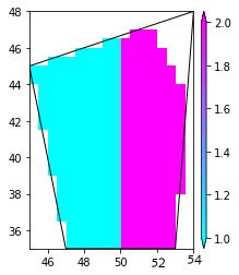
2.8 Result display

showraster2(r'tif_mask.tif',r'simple_mask.shp')

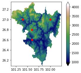
3 Extract grid data based on points

3.1 The first method

import geopandas
import rasterio
import matplotlib.pyplot as plt
from shapely.geometry import Point
# Create sampling points
points = [Point(101.4, 27.0), Point(101.6,26.6), Point(101.6,26.8), Point(102.0,27)]
gdf = geopandas.GeoDataFrame([1, 2, 3, 4], geometry=points, crs=4326)
src = rasterio.open(r'C:\Users\lenovo\Desktop\pzh_map_dispose\sf1.tif','r')
result1=src.read()
#If the conditions are met, replace it; otherwise, keep it as it is
result=np.where(result1==result1.min(),np.nan,result1)
result
# np.unique(rss[0])
from rasterio.plot import show
from matplotlib import colors, cm
fig, ax = plt.subplots()
# # transform rasterio plot to real world coords
# extent=[src.bounds[0], src.bounds[2], src.bounds[1], src.bounds[3]]
ax = rasterio.plot.show(src,ax=ax, cmap='gist_earth')
gdf.plot(ax=ax,color='red')
​​​​​​​fig.colorbar(cm.ScalarMappable(norm=colors.Normalize(vmin=np.nanmin(result), vmax=np.nanmax(result)), cmap='gist_earth', ax=ax,extend='both',fraction=0.05))

coord_list = [(x,y) for x,y in zip(gdf['geometry'].x , gdf['geometry'].y)]
coord_list
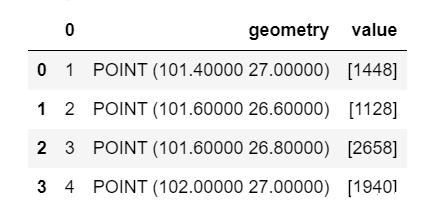
gdf['value'] = [x for x in src.sample(coord_list)]
gdf.head()

3.2 The second method

from rasterstats import gen_point_query
pointData=gdf
point_raster_value=gen_point_query(pointData['geometry'],r'C:\Users\lenovo\Desktop\pzh_map_dispose\sf1.tif')
print(*point_raster_value)